
코딩하는 해맑은 거북이
[Pandas] Pandas 기본 문법 본문
해당 글의 내용은 아래의 2개 주소의 내용에서 Pandas만 한번에 보기 쉽게 하기 위해 모은 것 입니다.
해당 글은 아래의 2가지를 다룬다.
1. Pandas I
🔹 pandas
🔹 Series
🔹 DataFrame
🔹 selection & drop
🔹 dataframe operations
🔹 lambda, map, apply
🔹 pandas built-in functions
2. Pandas II
🔹 Groupby I
🔹 Groupby II
🔹 Case Study
🔹 Pivot table & Crosstab
🔹 Merge & Concat
🔹 persistence
원본글 링크보기 ↓
인공지능(AI) 기초 다지기 (8)
본 게시물의 내용은 '인공지능(AI) 기초 다지기(부스트코스)' 강의를 듣고 작성하였다. 해당 글은 4-1. Pandas I / 딥러닝 학습방법 이해하기 2가지 파트를 다룬다. 1. Pandas I 2. 딥러닝 학습방법 이해하
cje1125.tistory.com
인공지능(AI) 기초 다지기 (9)
본 게시물의 내용은 '인공지능(AI) 기초 다지기(부스트코스)' 강의를 듣고 작성하였다. 해당 글은 4-2. Pandas II / 확률론 맛보기 2가지 파트를 다룬다. 1. Pandas II 2. 확률론 맛보기 1. Pandas II Groupby I ▶
cje1125.tistory.com
1. Pandas I
🔹 pandas
- 구조화된 데이터의 처리를 지원하는 Python 라이브러리, Python계의 엑셀!
- panel data의 줄임말 → pandas
- 고성능 array 계산 라이브러리인 numpy와 통합하여, 강력한 "스프레드시트" 처리 기능을 제공한다.
- 인덱싱, 연산용 함수, 전처리 함수 등을 제공한다.
- 데이터 처리 및 통계 분석을 위해 사용한다.
cf) 테이블 정의 예시
Data table, Sample : 전체 테이블
attribute, field, feature, column : 첫 번째 행
instance, tuple, row : 첫 번째 행이 아닌 의미있는 값을 가진 행
Feature vector : 하나의 feature에 있는 열 값들 (잘안씀)
data : 값, value
*pandas 설치 + 주피터 실행하기
conda create -n (가상환경이름) python=3.8	# 가상환경생성
activate (가상환경이름)	# 가상환경실행
conda install pandas	# pandas 설치
jupyter notebook # 주피터 실행하기
*데이터 로딩
- 라이브러리 호출
import pandas as pd # 라이브러리 호출- 데이터 url 불러오고 pd.read_csv() 함수를 통해 DataFrame 생성하기
# Data URL
data_url = 'https://archive.ics.uci.edu/ml/machine-learning-databases/housing/housing.data'
# pd.read_csv() : csv 타입 데이터 로드, separate는 빈공간으로 지정하고, Column은 없음
df_data = pd.read_csv(data_url, sep='\s+', header = None)
- DataFrame의 처음 5줄 출력하기
괄호 안에 n=??으로 몇 번째 줄까지 출력할 건지 설정 가능
df_data.head() # 처음 다섯줄 출력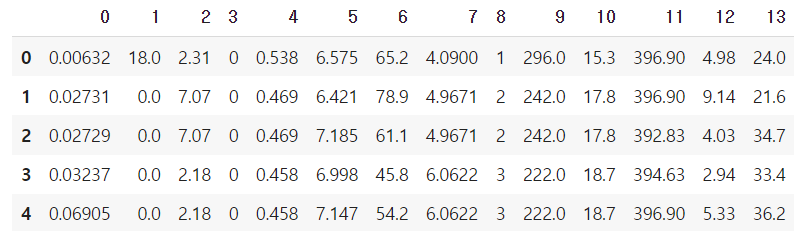
- Column Header 이름 지정
# Column Header 이름 지정
df_data.columns = [
    'CRIM','ZN', 'INDUS', 'CHAS', 'NOX', 'RM', 'AGE', 'DIS', 'RAD', 'TAX', 'PTRATIO' ,'B', 'LSTAT', 'MEDV']
df_data.head()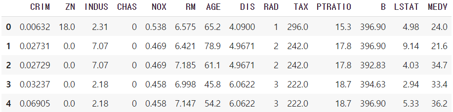
cf) pandas의 구성
DataFrame : DataTable 전체를 포함하는 Object
Series : DataFrame 중 하나의 Column에 해당하는 데이터의 모음 Object
🔹 Series
- Column vector를 표현하는 Object
- numpy.ndarray의 Subclass 이다.
- index 값을 숫자 또는 문자로도 지정가능하다.
- duplicates 가능
- 라이브러리 호출
from pandas import Series, DataFrame
import pandas as pd
import numpy as np
- series 생성
list_data = [1,2,3,4,5]
example_obj = Series(data = list_data)
example_obj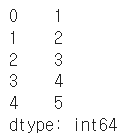
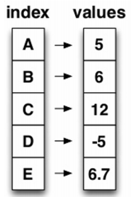
- 리스트로 index 이름을 지정
list_data = [1,2,3,4,5]
list_name = ["a","b","c","d","e"]
example_obj = Series(data = list_data, index=list_name)
example_obj
- 딕셔너리로 data와 index 이름을 지정
Series 함수 - dtype : data type설정 / name : series 이름 설정
dict_data = {"a":1, "b":2, "c":3, "d":4, "e":5}
example_obj = Series(dict_data, dtype=np.float32, name="example_data")
example_obj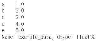
- data index에 접근하기
example_obj["a"]
- data index에 값 할당하기 & 타입 변형
example_obj = example_obj.astype(float) # 타입 변형
example_obj["a"] = 3.2
example_obj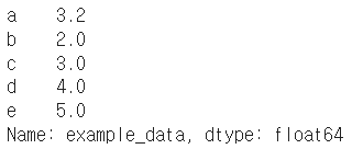
- value가 2보다 큰 값 출력하기
cond = example_obj > 2
example_obj[cond]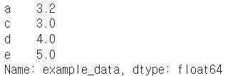
cf) 이외 연산들
example_obj * 2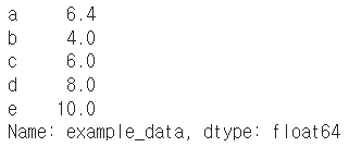
np.exp(example_obj) #np.abs , np.log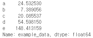
- series에 특정 index가 있는지 확인
"b" in example_obj
- series를 dict로 변형 : to_dict()
example_obj.to_dict()
- value 리스트 출력
example_obj.values
- index 리스트 출력
example_obj.index
- data에 대한 정보를 저장
(Series).name : series 이름 설정
(Series).index.name : series의 index 이름 설정
example_obj.name = "number"
example_obj.index.name = "alphabet"
example_obj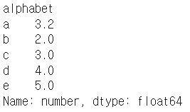
- index 값을 기준으로 series 생성
dict_data_1 = {"a":1, "b":2, "c":3, "d":4, "e":5}
indexes = ["a","b","c","d","e","f","g","h"]
series_obj_1 = Series(dict_data_1, index=indexes)
series_obj_1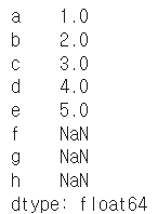
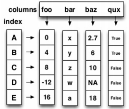
🔹 DataFrame
- Series를 모아서 만든 Data Table = 기본 2차원
- DataFrame에 있는 하나의 값을 알기 위해서는 index와 columns를 모두 알아야한다.
- 각각의 값들의 데이터 타입이 다를 수 있다.
- 라이브러리 호출
from pandas import Series, DataFrame
import pandas as pd
import numpy as np
- dict 형태로 저장된 데이터를 columns로 불러 df 생성하기
# Example from - https://chrisalbon.com/python/pandas_map_values_to_values.html
raw_data = {'first_name': ['Jason', 'Molly', 'Tina', 'Jake', 'Amy'],
        'last_name': ['Miller', 'Jacobson', 'Ali', 'Milner', 'Cooze'],
        'age': [42, 52, 36, 24, 73],
        'city': ['San Francisco', 'Baltimore', 'Miami', 'Douglas', 'Boston']}
df = pd.DataFrame(raw_data, columns = ['first_name', 'last_name', 'age', 'city'])
df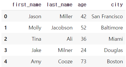
* 일부 columns 만 불러오기
DataFrame(raw_data, columns = ["age", "city"])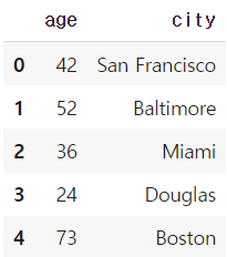
* dict에 없는 key값 불러올 시 NaN으로 저장
DataFrame(raw_data, columns = ["first_name","last_name","age", "city", "debt"])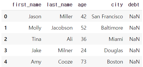
- series 추출 방법 2가지
df = DataFrame(raw_data, columns = ["first_name","last_name","age", "city", "debt"])
df.first_name   # Series 추출 방법1
df["first_name"] # Series 추출 방법2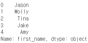
* 타입 참고!
type(df["first_name"])
- dataframe indexing
* loc : index location
* iloc : index position / index값을 0부터 할당하는 것 처럼 봄
df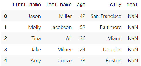
df.loc[1]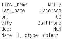
df["age"].iloc[1:]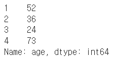
df.loc[:3]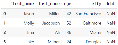
df.loc[:, ["first_name", "last_name"]] # 뒤에는 리스트 형태로 넣어줘야함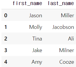
* loc는 index 이름, iloc은 index number
# Example from - https://stackoverflow.com/questions/31593201/pandas-iloc-vs-ix-vs-loc-explanation
s = pd.Series(np.nan, index=[49,48,47,46,45, 1, 2, 3, 4, 5])
s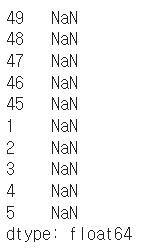
s.loc[:3]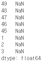
s.iloc[:3]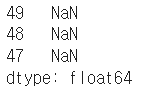
- dataframe handling
* column에 새로운 데이터 할당
df.debt = df.age > 40
df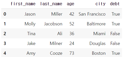
values = Series(data=["M","F","F"],index=[0,1,3])
values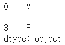
df["sex"] = values
df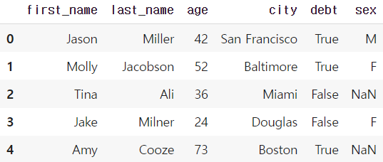
* Transpose
df.T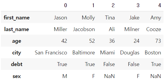
df.head(3).T
* 값 출력
df.values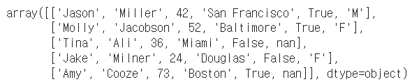
* csv 변환 : to_csv()
df.to_csv()
* 일부 column 을 drop한 상태로 출력
df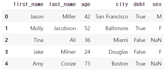
df.drop("debt", axis=1) # df자체에는 삭제되지 않고, drop만 된 상태로 출력됨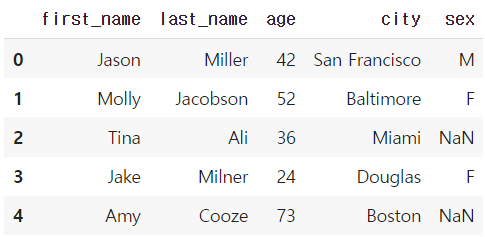
* column 삭제
del df["debt"] # 메모리 주소가 삭제되면서 아예 삭제되는 것.
cf) json파일 형태에서 종종 볼 수 있음 (보통의 경우엔 잘안씀)
# Example from Python for data analyis
pop = {'Nevada': {2001: 2.4, 2002: 2.9}, 'Ohio': {2000: 1.5, 2001: 1.7, 2002: 3.6}}
DataFrame(pop)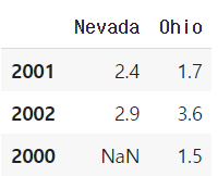
🔹 selection & drop
- 엑셀 파일 가져오기 & 읽기
여기서는 구글 코랩 드라이브 마운트를 이용하여 엑셀파일을 가져왔다.
from google.colab import drive
drive.mount('/content/drive')
import numpy as np
df = pd.read_excel("/content/drive/My Drive/excel-comp-data.xlsx")
df.head()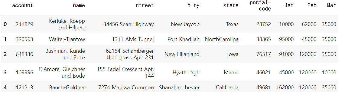
df.head(2).T # 데이터를 좀더 명확하게 보기위해 transpose를 사용하기도 한다!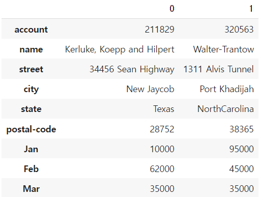
- Selection with column names
1) 1개의 column 선택시
df["account"].head(2) # Series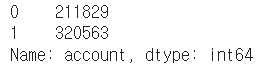
df[["account"]].head(2) # DF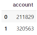
2) 1개 이상의 column 선택시
df[["account", "street", "state"]].head(3)
- Selection with index number
1) column 이름 없이 사용하는 index number는 row 기준 표시
df[:3]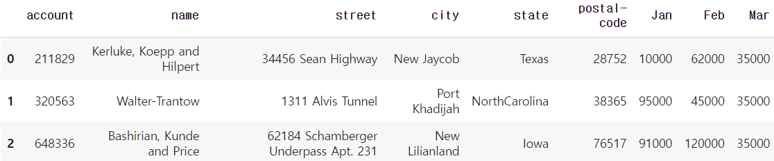
2) column 이름과 함께 row index 사용시, 해당 column만 출력
df["account"][:3]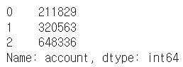
account_serires = df["account"]
account_serires[:3]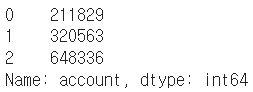
account_serires[[0,1,2]]
account_serires[account_serires<250000] # Boolean index, True인 값만 출력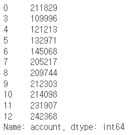
account_serires[list(range(0, 15, 2))]
- index 변경
df.index = df["account"]
df.head()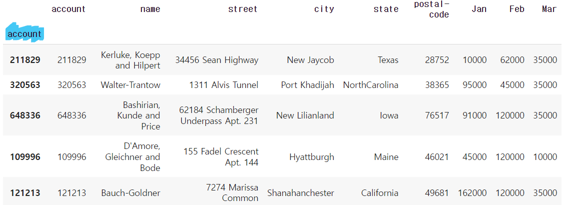
del df["account"]		# "account" column 삭제
df.head()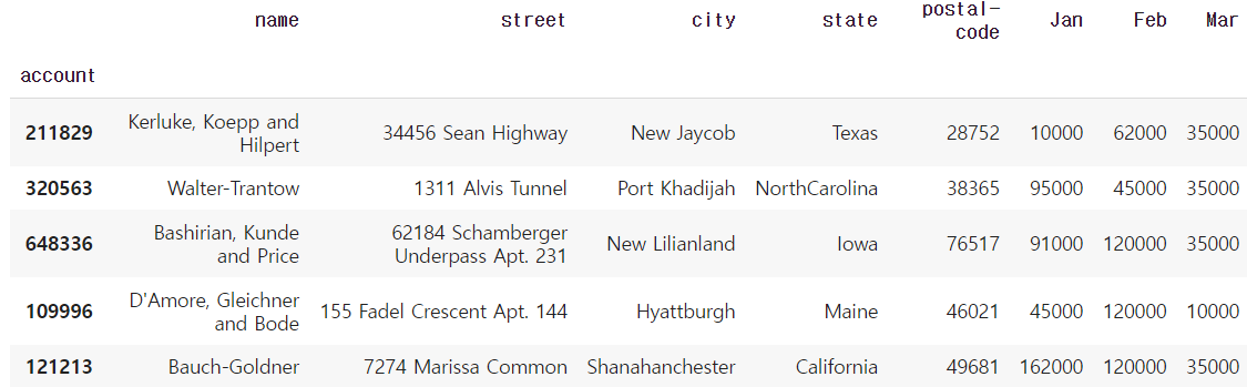
- basic, loc, iloc selection
1) Column과 index number
df[["name","street"]][:2]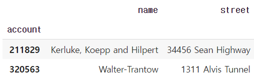
df[["name", "street"]].iloc[:10]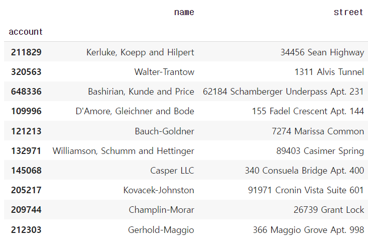
2) Column과 index name
df.loc[[211829,320563],["name","street"]]
3) Column number와 index number
df.iloc[:2,:2]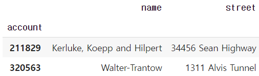
- index 재설정
1) index 값 다시 설정
df.index = list(range(0,15))    # reindex
df.head()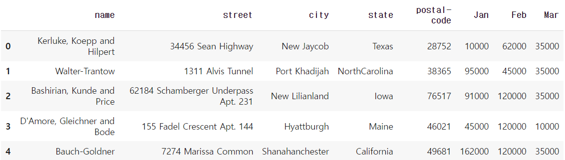
2) 기존 index가 사라지고 새로운 index가 생성된 DF 출력, DF 자체는 변경되지않음!
df.reset_index(drop=True) # 기존 index가 사라지고 새로운 index 생성된 DF 출력, DF 자체는 변경X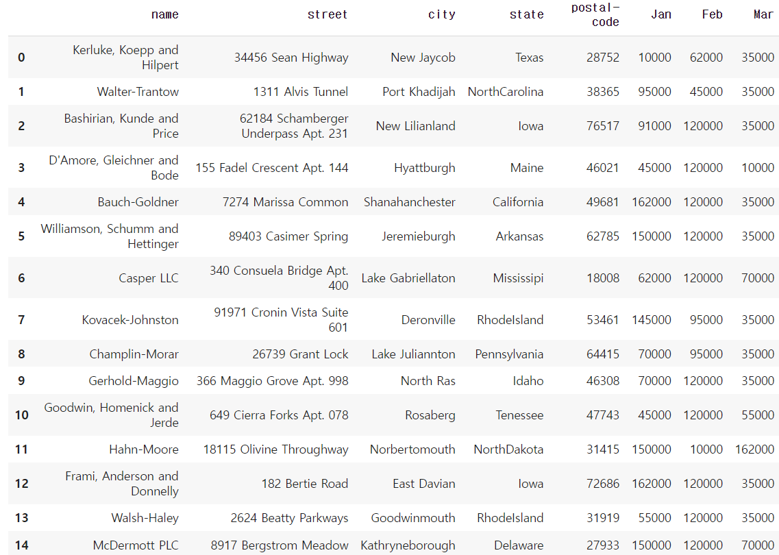
* DF 자체도 변경하는 방법
여기서 drop을 True로 설정하지 않았으므로, 기존 index는 column으로 추가되었다.
df.reset_index(inplace=True)   # inplace=True로 설정해서 DF가 변경됨
df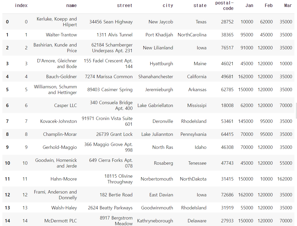
- data drop
df.drop(index number) : DF 자체는 변경되지 않음!
1) index number로 drop
df.drop(1)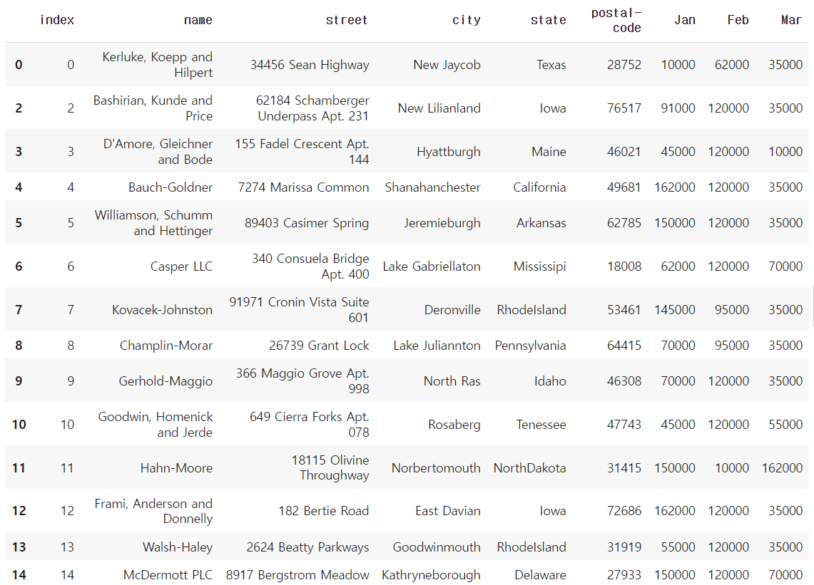
2) 한 개 이상의 index number로 drop
df.drop([0, 1, 2, 3])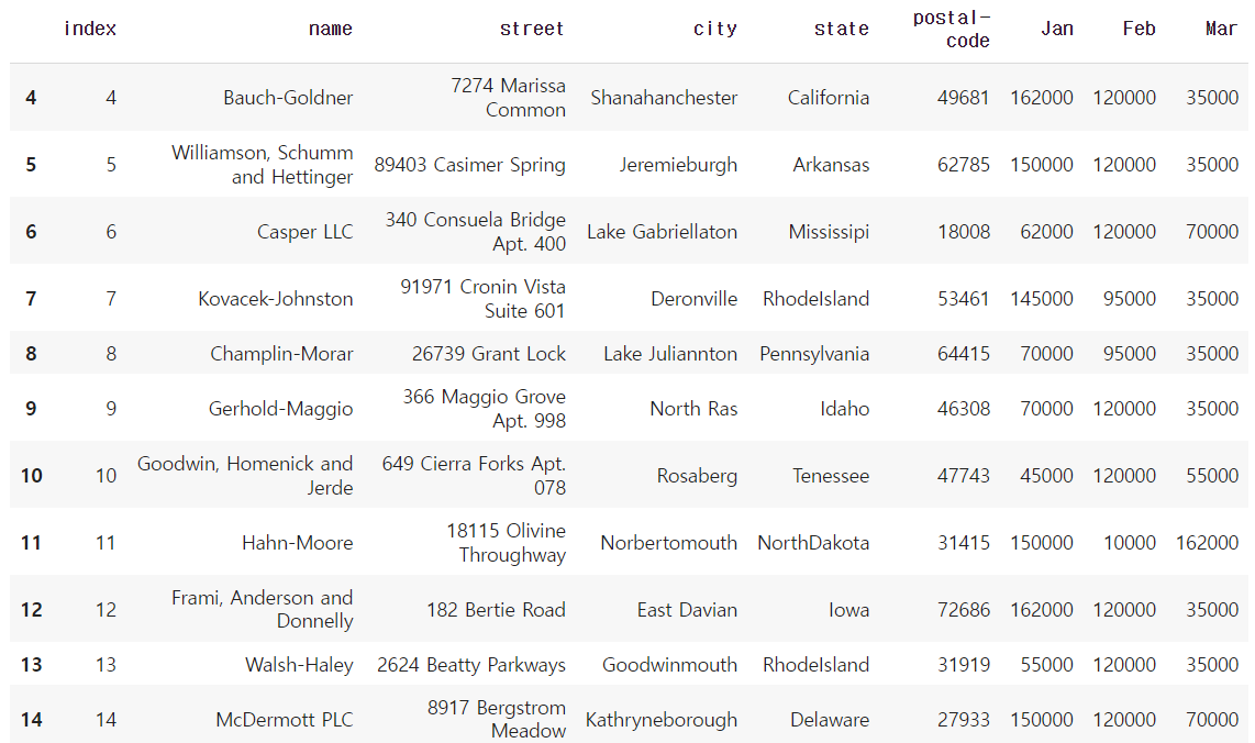
3) axis 지정으로 축을 기준으로 drop → column 중에 "city"
df.drop("city",axis=1)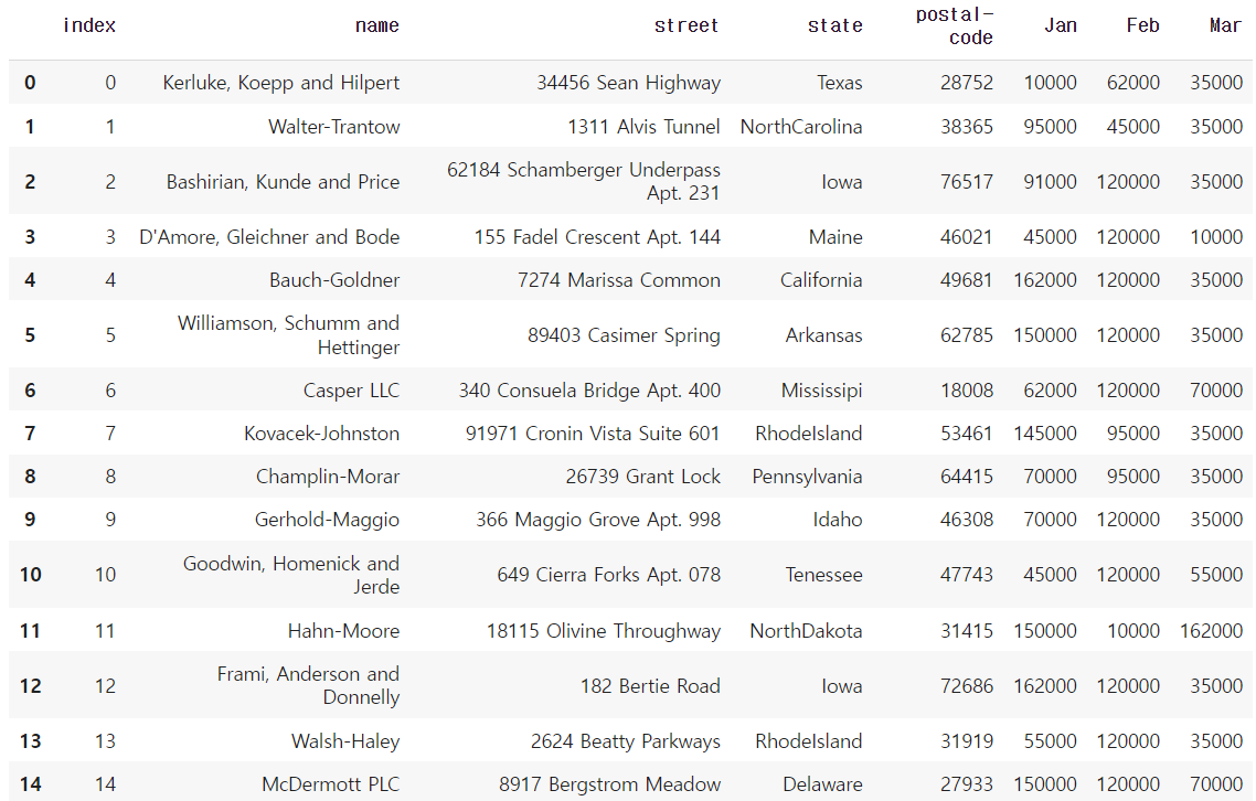
- dataframe의 값을 numpy 형태로 데이터 생성
matrix = df.values
matrix[:3]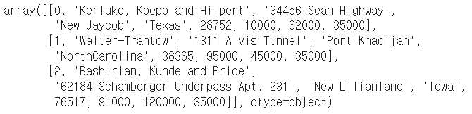
matrix[:,-3:]
matrix[:,-3:].sum(axis=1)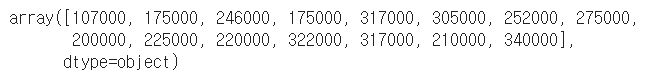
df.drop("index", axis=1, inplace=True)
df
matrix = df.values
matrix      # numpy 형태로 데이터를 뽑아낼 수 있음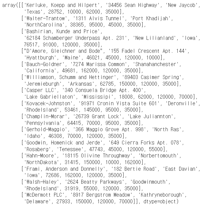
🔹 dataframe operations
- series operation
index를 기준으로 연산을 수행한다. 겹치는 index가 없을 경우 NaN 값으로 반환한다.
s1 = Series(range(1,6), index=list("abced"))
s1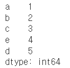
s2 = Series(range(5,11), index=list("bcedef"))
s2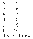
s1 + s2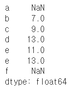
s1.add(s2)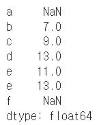
- dataframe operation
dataframe은 column과 index를 모두 고려한다.
add operation을 쓸 때 fill_value를 0으로 설정하면 NaN 값을 0으로 변환하여 계산한다.
mul operation을 쓸 때 fill_value를 1으로 설정하면 NaN 값을 1으로 변환하여 계산한다.
* operation types : add, sub, div, mul
df1 = DataFrame(np.arange(9).reshape(3,3), columns=list("abc"))
df1
df2 = DataFrame(np.arange(16).reshape(4,4), columns=list("abcd"))
df2
df1 + df2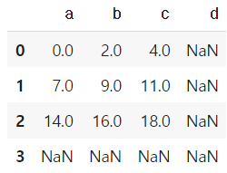
df1.add(df2)
df1.add(df2,fill_value=0)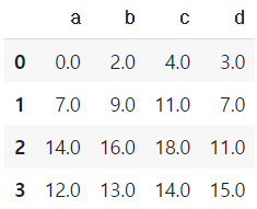
df1.mul(df2,fill_value=1)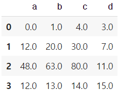
- series + dataframe
기본 연산은 df의 column과 series의 index로 column broadcasting이 일어난다.
row broadcasting 실행하기 위해선 axis를 0으로 두면 된다.
df = DataFrame(np.arange(16).reshape(4,4), columns=list("abcd"))
df
s = Series(np.arange(10,14), index=list("abcd"))
s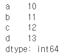
df + s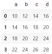
s2 = Series(np.arange(10,14))
s2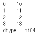
df + s2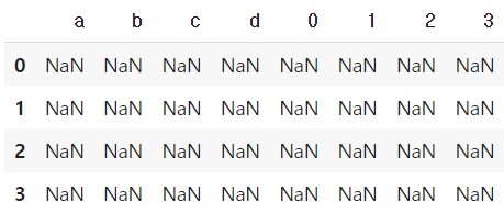
df.add(s2, axis=0)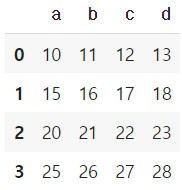
🔹 lambda, map, apply
- map for series
pandas의 series type의 데이터에도 map 함수 사용가능
function 대신 dict, sequence형 자료 등으로 대체 가능
s1 = Series(np.arange(10))
s1.head(5)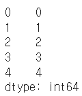
s1.map(lambda x: x**2).head(5)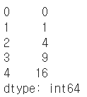
# f = lambda x: x+5   # lambda function
def f(x):
  return x+5
s1.map(f)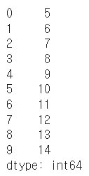
z = {1: 'A', 2: 'B', 3: 'C'}
s1.map(z)		# dict type으로 데이터 교체, 없는값은 NaN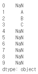
s2 = Series(np.arange(10,20))
s1.map(s2)		# 같은 위치의 데이터를 s2로 전환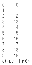
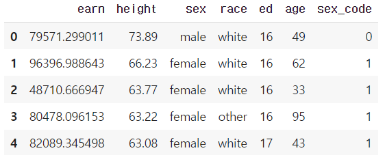
* example
df = pd.read_csv("./wages.csv")
df.head()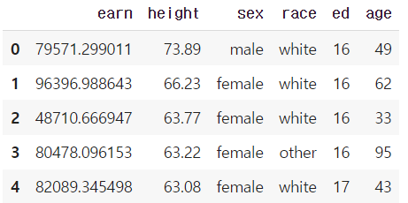
df.sex.unique() # series data의 유일한 값을 list로 반환함
df["sex_code"] =  df.sex.map({"male":0, "female":1})  # 매핑 : 성별 str -> 성별 code
df.head(5)
def change_sex(x):
  return 0 if x == "male" else 1
df.sex.map(change_sex).head()		# df 자체는 변경X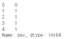
- replace function
Map 함수의 기능 중 데이터 변환 기능만 담당
데이터 변환시 많이 사용하는 함수
df.sex.replace(
    {"male":0, "female":1}		# dict type 적용
).head()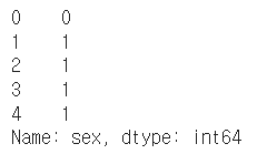
df.sex.head(5) # df 자체가 변경되지 않음!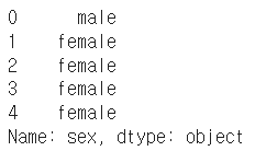
df.sex.replace(
    ["male", "female"], 	# target list
    [0,1], inplace=True)    # conversion list
# df 자체를 바꾸기 위해서는 inplace를 넣어줘야한다! inplace는 데이터 변환결과를 적용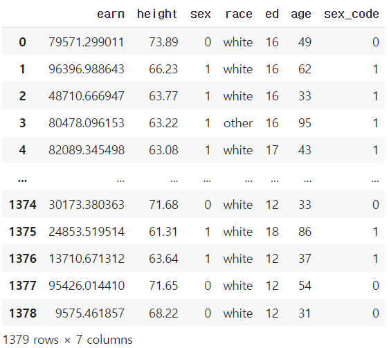
- apply for dataframe
map과 달리 series 전체(column)에 해당 함수를 적용한다.
입력 값이 series 데이터로 입력 받아 handling 가능하다. → 각 column 별로 결과값 반환
내장 연산 함수를 사용할 때도 똑같은 효과를 거둘 수 있다. (mean, std 등)
scalar 값 이외에 series 값의 반환도 가능하다.
df_info = df[["earn", "height","age"]]
df_info.head()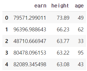
f = lambda x : x.max() - x.min()
df_info.apply(f)    # series 데이터로 입력받아 handling  가능
df_info.apply(sum)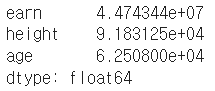
df_info.sum()
def f(x):
    return Series([x.min(), x.max(), x.mean(), sum(x.isnull())],
                    index=["min", "max", "mean", "null"])
df_info.apply(f)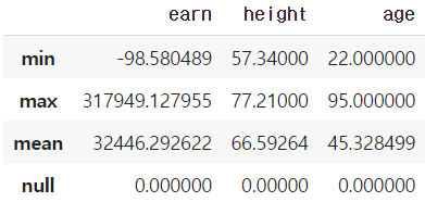
- applymap for dataframe
series 단위가 아닌 element 단위로 함수를 적용한다.
series 단위에 apply를 적용시킬 때와 같은 효과
f = lambda x : -x
df_info.applymap(f).head(5)   # 모든 값에 적용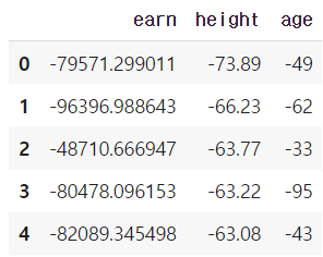
f = lambda x: x//2
df_info.applymap(f).head(5)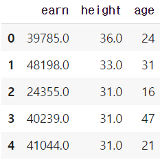
f = lambda x : -x
df_info["earn"].apply(f).head(5)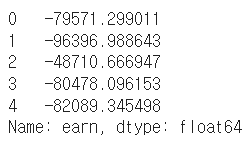
🔹 pandas built-in functions
df = pd.read_csv("./wages.csv")
df.head()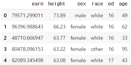
- describe
Numeric type 데이터의 요약 정보를 보여준다.
df.describe()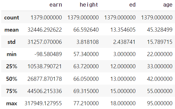
- unique
series data의 유일한 값을 list로 반환한다.
unique 함수를 사용해서 라벨 인코딩을 할 수 있다.
df.race.unique()
dict(enumerate(sorted(df["race"].unique())))
# 라벨인코딩1
key = df.race.unique()
value = range(len(df.race.unique()))
df["race"].replace(to_replace=key, value=value)	# df자체변경X, inplace 설정해야 변경된다.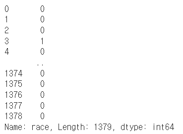
# 라벨인코딩2
value = list(map(int, np.array(list(enumerate(df["race"].unique())))[:, 0].tolist()))
key = np.array(list(enumerate(df["race"].unique())), dtype=str)[:, 1].tolist()

value, key
df["race"].replace(to_replace=key, value=value, inplace=True)
df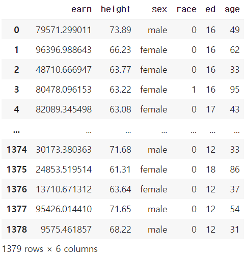
# 라벨인코딩2 - label str인 sex에 대해서도 index 값으로 변환
value = list(map(int, np.array(list(enumerate(df["sex"].unique())))[:, 0].tolist()))
key = np.array(list(enumerate(df["sex"].unique())), dtype=str)[:, 1].tolist()

value, key
df["sex"].replace(to_replace=key, value=value, inplace=True)
df.head(5)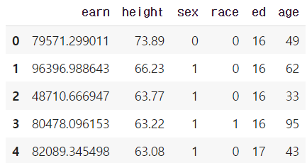
- sum
기본적인 column 또는 row 값의 연산을 지원한다.
(sub, mean, min, max, count, median, mad, var 등)
df.sum(axis=1)
df.sum(axis=0)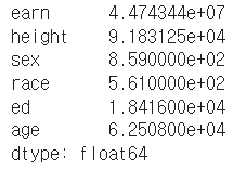
numueric_cols = ["earn", "height", "ed", "age"]   # 숫자데이터만 뽑아서 sum
df[numueric_cols].sum(axis=1)	# row별 sum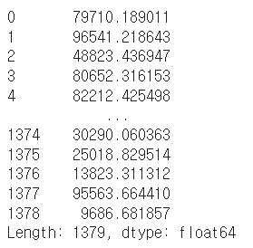
df[numueric_cols].sum(axis=0) # column별 sum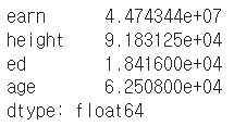
- isnull
column 또는 row 값의 NaN (null) 값의 index를 반환함
df.isnull() # null 인지 아닌지 True or False로 반환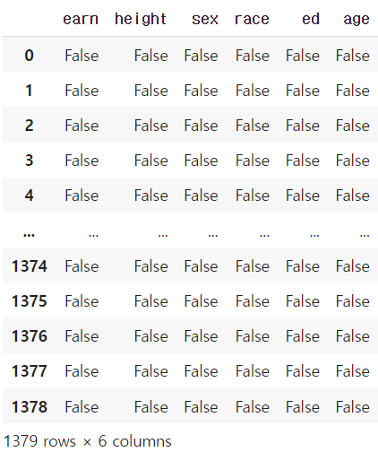
df.isnull().sum() # null인 값의 합
df.isnull().sum() / len(df) # null을 가진 비율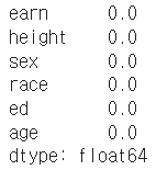
- pd.options.display.max_rows
한번에 보여줄 수 있는 행의 크기를 조절할 수 있다.
pd.options.display.max_rows = 2000 # 한번에 보여줄수있는 행의 크기를 조절할 수 있음
- sort_values
column 값을 기준으로 데이터를 sorting
ascending은 오름차순을 의미한다.
df.sort_values(["age", "earn"], ascending=False).head(10)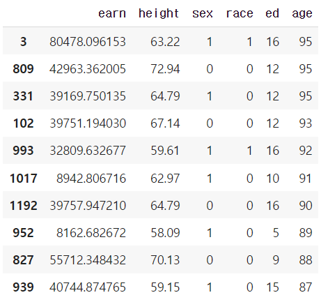
df.sort_values("age", ascending=False).head(10)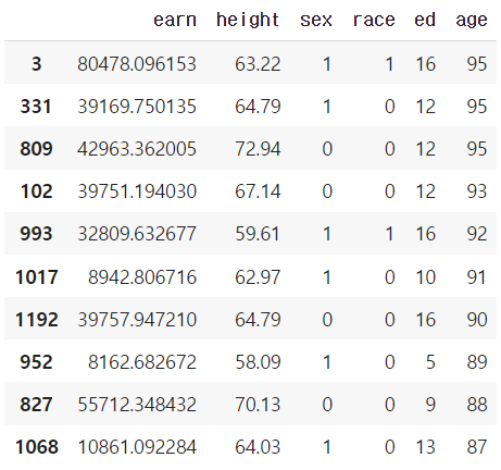
- cumsum & cummax 등 누적값 구하기
df.cumsum().head(5)
df.cummax().head(10)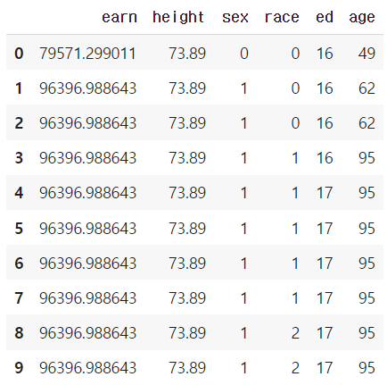
- Correlation & Covariance
상관계수와 공분산을 구하는 함수 (corr, cov, corrwith)
df.age.corr(df.earn)
df.age[(df.age<45) & (df.age>15)].corr(df.earn)
df.age.cov(df.earn)
df.corr() # 모든 column 간에 corr 을 보여줌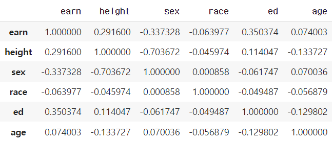
df.corrwith(df.earn) # earn 값과 전체 값과의 corr 계산된 걸 보여줌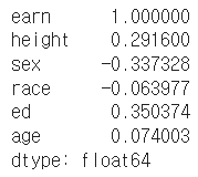
- value_counts
특정 column의 값의 빈도수를 보여준다.
df.sex.value_counts(sort=True) # 글자의 갯수가 몇개인지
df.sex.value_counts(sort=True) / len(df) # 글자의 갯수에 따른 비율로 보여줌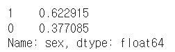
2. Pandas II
🔹 Groupby I
▶ Groupby
- df.groupby(묶음의 기준이 되는 컬럼)[적용받는 컬럼].적용받는연산()
- SQL groupby 명령어와 같음
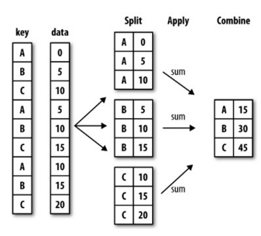
- split → apply → combine
- 과정을 거쳐 연산함
# 예제 데이터
ipl_data = {'Team': ['Riders', 'Riders', 'Devils', 'Devils', 'Kings',
         'kings', 'Kings', 'Kings', 'Riders', 'Royals', 'Royals', 'Riders'],
         'Rank': [1, 2, 2, 3, 3,4 ,1 ,1,2 , 4,1,2],
         'Year': [2014,2015,2014,2015,2014,2015,2016,2017,2016,2014,2015,2017],
         'Points':[876,789,863,673,741,812,756,788,694,701,804,690]}

df = pd.DataFrame(ipl_data)
df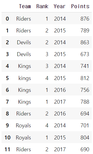
df.groupby("Team")["Points"].sum()
df.groupby("Team")["Points"].mean()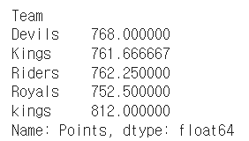
▶ Hierarchical index
- Groupby 명령의 결과물도 결국은 dataframe
- 두 개의 column으로 groupby를 할 경우, index가 두 개 생성된다.
- 한 개 이상의 column을 묶을 수 있음. 이때 2개의 index가 구성된 것을 Hierarchical index라고 부른다.
h_index = df.groupby(["Team", "Year"])["Points"].sum()
h_index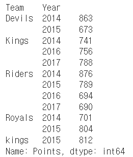
h_index.index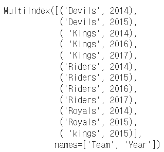
h_index["Devils":"Kings"]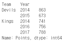
- unstack()
Group으로 묶어진 데이터를 matrix 형태로 전환해줌
h_index.unstack()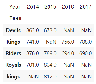
h_index.unstack().stack() # stack() 함수로 되돌릴수도 있음
- reset_index()
index를 없애주면서 풀어서 보여주는 함수
h_index.reset_index() # index를 없애주면서 풀어서 보여준다.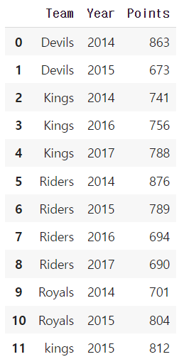
- swaplevel()
index level을 변경할 수 있음, 아래의 예제에서 "Year"과 "Team"의 위치가 바뀐 것을 볼 수 있다.
h_index.swaplevel()
sort_index(level=0) 함수를 통해 "Year" index를 기준으로 sort 할 수 있다.
h_index.swaplevel().sort_index(level=0)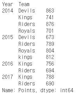
- sort_values()
연산된 값을 기준으로 정렬해서 보여준다.
h_index.sort_values()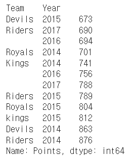
Q. h_index의 타입은? Series
index가 2개 있다고해서 DF가 아니라 Series이다.
type(h_index)
- operations
index level을 기준으로 기본 연산 수행 가능하다.
h_index.sum(level=0)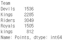
h_index.sum(level=1)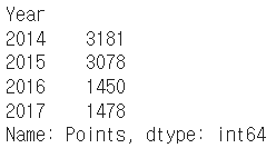
🔹 Groupby II
▶ grouped
Groupby에 의해 split된 상태를 추출 가능하다.
→ Tuple 형태로 그룹의 key, value 값이 추출된다.
grouped = df.groupby("Team")for name,group in grouped:
print (name)
print (group)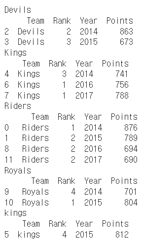
Q. group의 타입은? DataFrame
type(group)
특정 key값을 가진 그룹의 정보만 추출 가능 : get_group()
grouped.get_group("Devils")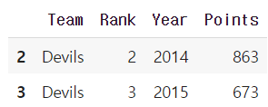
* 추출된 group 정보에는 세 가지 유형의 apply가 가능함
- Aggregation: 요약된 통계정보를 추출해 줌
- Transformation: 해당 정보를 변환해줌
- Filtration: 특정 정보를 제거 하여 보여주는 필터링 기능
▶ Aggregation
column 별로 연산을 해주되, group별로 데이터를 출력해준다.
grouped.agg(sum)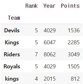
grouped.agg(max)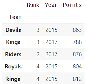
import numpy as np
grouped.agg(np.mean)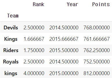
특정 column에 여러개의 function을 apply 할 수 도 있음
grouped['Points'].agg([np.sum, np.mean, np.std])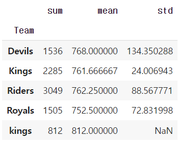
▶ transformation
Aggregation과 달리 key 값 별로 요약된 정보가 아니다!
개별 데이터의 변환을 지원한다.
transform : grouped된 상태에서 모든 값을 다 지정해주는 함수이다.
단, max나 min 처럼 Series 데이터에 적용되는 데이터들은 key값을 기준으로 Grouped된 데이터 기준
df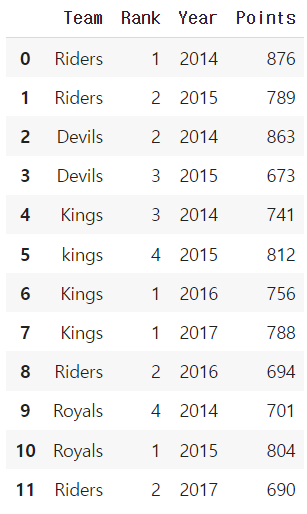
score = lambda x: (x.max())
grouped.transform(score)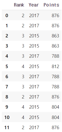
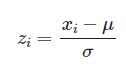
score = lambda x: (x - x.mean()) / x.std()
grouped.transform(score)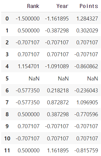
▶ filter
특정 조건으로 데이터를 검색할 때 사용한다.
df["Team"].value_counts()
df.groupby('Team').filter(lambda x: len(x) >= 3) # 위의 결과로 봤을때 3이상 인 건 Riders, Kings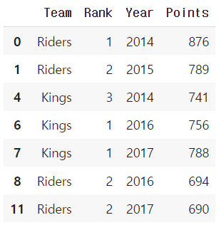
df.groupby('Team').filter(lambda x: x["Points"].max() > 800)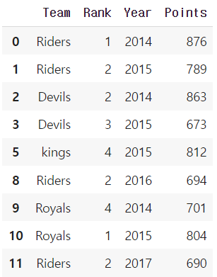
🔹 Case Study
- 원래 통화량 데이터
df_phone = pd.read_csv("phone_data.csv")
df_phone.head()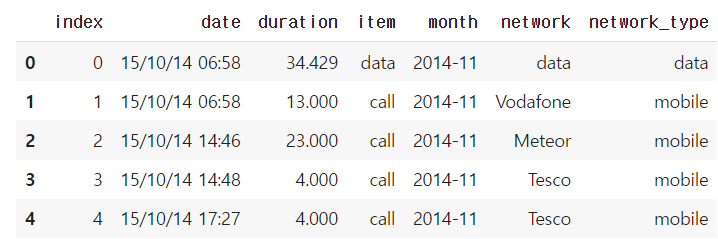
df_phone.dtypes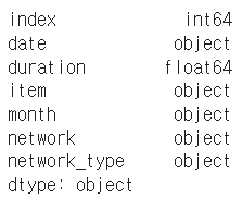
- 시간과 데이터 종류가 정리된 통화량 데이터
# 문자 형태의 date를 datetime 타입으로 변경해주기
import dateutil
df_phone['date'] = df_phone['date'].apply(dateutil.parser.parse, dayfirst=True)
df_phone.head()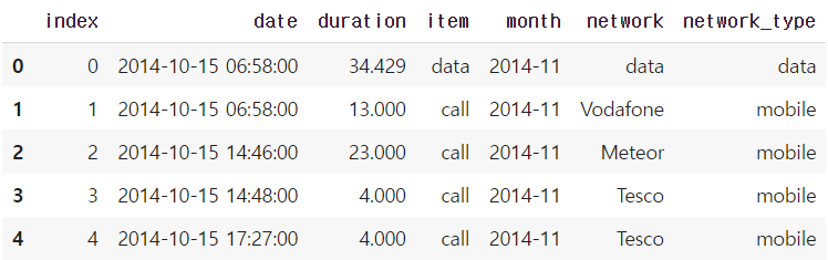
df_phone.dtypes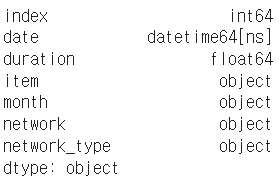
df_phone.groupby('month')['duration'].sum()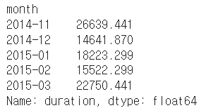
df_phone.groupby('month')['duration'].sum().plot() # 월별 통화량 그래프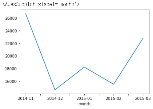
df_phone[df_phone['item'] == 'call'].groupby('month')['duration'].sum()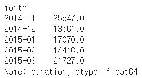
df_phone[df_phone['item'] == 'call'].groupby('month')['duration'].sum().plot()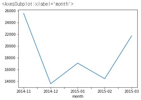
df_phone.groupby(['month', 'item'])['duration'].count()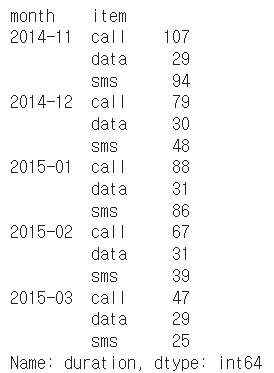
df_phone.groupby(['month', 'item'])['duration'].count().unstack().plot()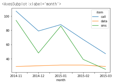
df_phone.groupby('month', as_index=False).agg({"duration": "sum"})
# as_index=False : 'month'를 index로 설정하지 않는다는 것.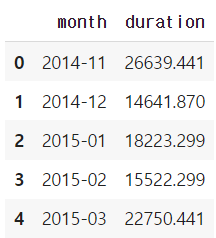
df_phone.groupby('month').agg({"duration": "sum"})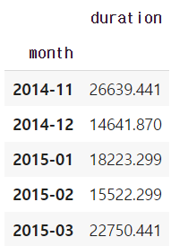
df_phone.groupby('month').agg({"duration": "sum"}).reset_index()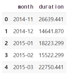
df_phone.groupby(['month', 'item']).agg({'duration':sum,      # find the sum of the durations for each group
                                     'network_type': "count", # find the number of network type entries
                                     'date': 'first'})    # get the first date per group
df_phone.groupby(['month', 'item']).agg({'duration': [min],      # find the min, max, and sum of the duration column
                                     'network_type': "count", # find the number of network type entries
                                     'date': [min, 'first', 'nunique']})    # get the min, first, and number of unique dates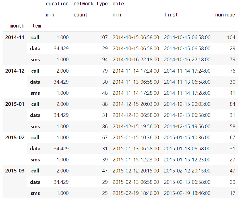
grouped = df_phone.groupby('month').agg( {"duration" : [min, max, np.mean]})
grouped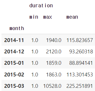
grouped.columns = grouped.columns.droplevel(level=0)
grouped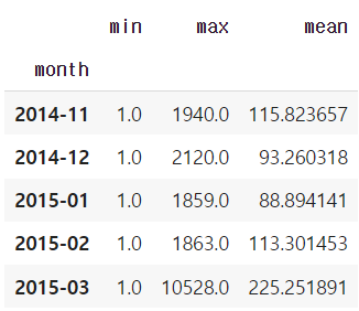
# column 이름 변경
grouped.rename(columns={"min": "min_duration", "max": "max_duration", "mean": "mean_duration"})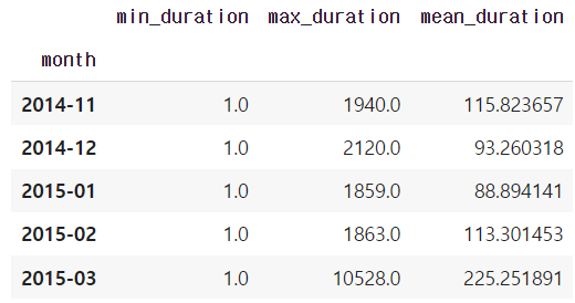
grouped = df_phone.groupby('month').agg( {"duration" : [min, max, np.mean]})
grouped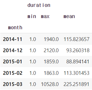
grouped.columns = grouped.columns.droplevel(level=0)
grouped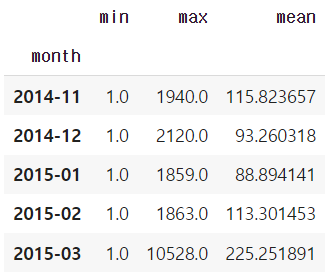
# 앞에 duration을 붙여줘서 어떤 column과 연산을 했는지 알아보기 쉽게 해줌
grouped.add_prefix("duration_")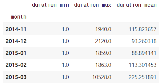
🔹 Pivot table & Crosstab
▶ Pivot Table
- 우리가 excel에서 보던 것
- Index축은 groupby와 동일함
- Column에 추가로 labeling값을 추가하여, Value에 numerictype값을 aggregation하는 형태
df_phone = pd.read_csv("phone_data.csv")
df_phone['date'] = df_phone['date'].apply(dateutil.parser.parse, dayfirst=True)
df_phone.head()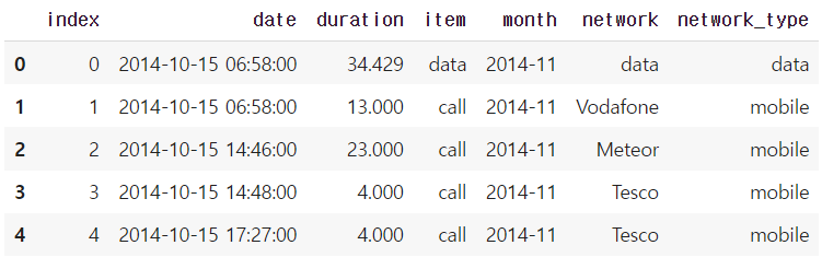
df_phone.pivot_table(values=["duration"],
                     index=[df_phone.month,df_phone.item],
                     columns=df_phone.network,
                     aggfunc="sum",
                     fill_value=0)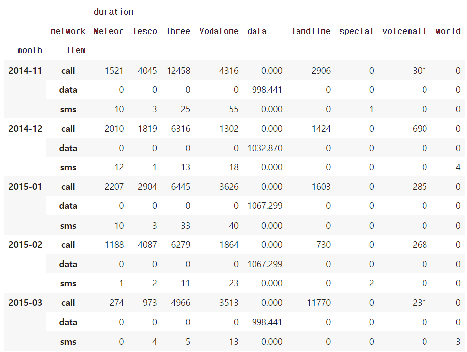
# 물론 groupby를 써도 비슷한 결과를 가져올 수 있음
df_phone.groupby(["month", "item", "network"])["duration"].sum().unstack()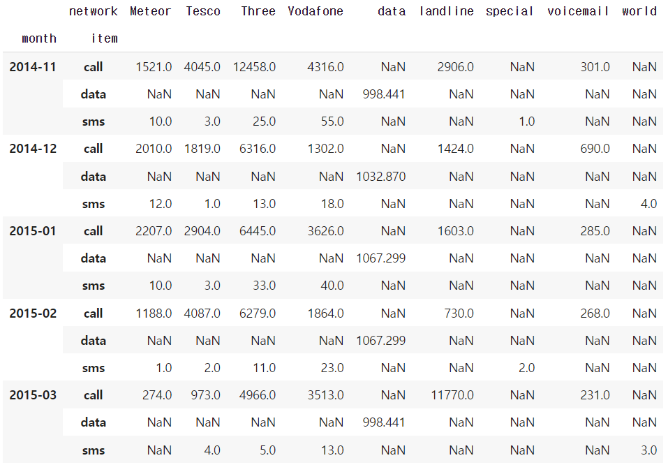
▶ Crosstab
- 특히 두 칼럼에 교차 빈도,비율,덧셈 등을 구할 때 사용
- Pivottable의 특수한 형태
- User-ItemRatingMatrix등을 만들 때 사용가능함
import numpy as np
df_movie = pd.read_csv("/content/drive/My Drive/movie_rating.csv")
df_movie.head()
df_movie.pivot_table(["rating"],
                     index=df_movie.critic,
                     columns=df_movie.title,
                     aggfunc="sum",
                     fill_value=0)
pd.crosstab(index=df_movie.critic,columns=df_movie.title,values=df_movie.rating,
            aggfunc="first").fillna(0)
df_movie.groupby(["critic","title"]).agg({"rating":"first"}).unstack().fillna(0)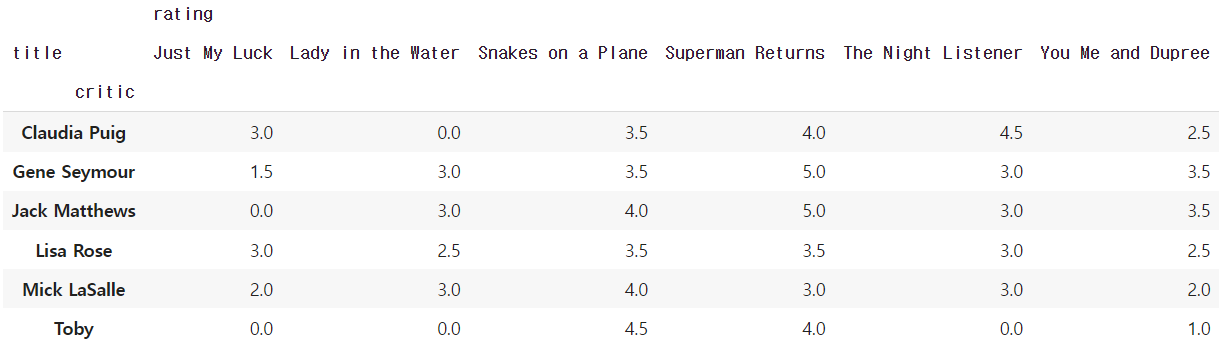
🔹 Merge & Concat
▶ Merge
- SQL에서 많이 사용하는 Merge와 같은 기능
- 두 개의 데이터를 하나로 합침
raw_data = {
        'subject_id': ['1', '2', '3', '4', '5', '7', '8', '9', '10', '11'],
        'test_score': [51, 15, 15, 61, 16, 14, 15, 1, 61, 16]}
df_a = pd.DataFrame(raw_data, columns = ['subject_id', 'test_score'])
df_a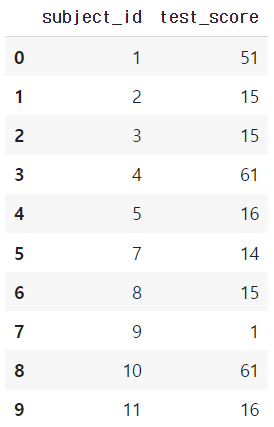
raw_data = {
        'subject_id': ['4', '5', '6', '7', '8'],
        'first_name': ['Billy', 'Brian', 'Bran', 'Bryce', 'Betty'],
        'last_name': ['Bonder', 'Black', 'Balwner', 'Brice', 'Btisan']}
df_b = pd.DataFrame(raw_data, columns = ['subject_id', 'first_name', 'last_name'])
df_b
- 두 dataframe의 column이 같을 때 : pd.merge(df_a, df_b, on='subject_id')
pd.merge(df_a, df_b, on='subject_id')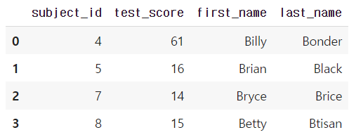
- 두 dataframe의 column이 다를 때 : pd.merge(df_a, df_b, left_on='subject_id', right_on='subject_id')
pd.merge(df_a, df_b, left_on='subject_id', right_on='subject_id')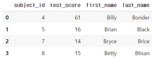
- join method

- left join
pd.merge(df_a, df_b, on='subject_id', how='left')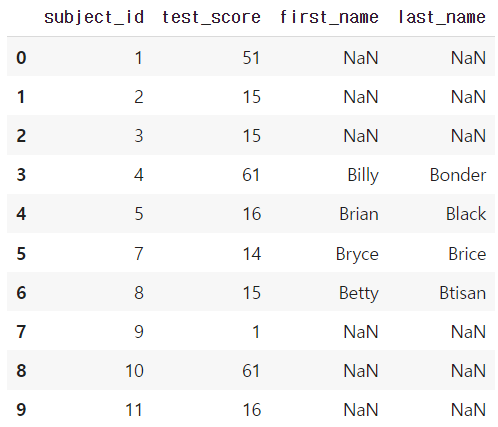
- right join
pd.merge(df_a, df_b, on='subject_id', how='right')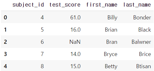
- full(outer) join
pd.merge(df_a, df_b, on='subject_id', how='outer')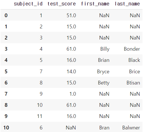
- inner join
default 가 inner join 이다.
pd.merge(df_a, df_b, on='subject_id', how='inner')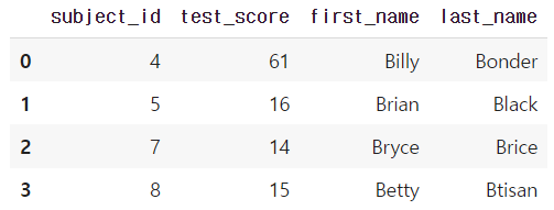
- inner based join
pd.merge(df_a, df_b, right_index=True, left_index=True)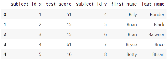
▶ Concat
- 같은 형태의 데이터를 붙이는 연산작업
raw_data = {
        'subject_id': ['1', '2', '3', '4', '5'],
        'first_name': ['Alex', 'Amy', 'Allen', 'Alice', 'Ayoung'],
        'last_name': ['Anderson', 'Ackerman', 'Ali', 'Aoni', 'Atiches']}
df_a = pd.DataFrame(raw_data, columns = ['subject_id', 'first_name', 'last_name'])
df_a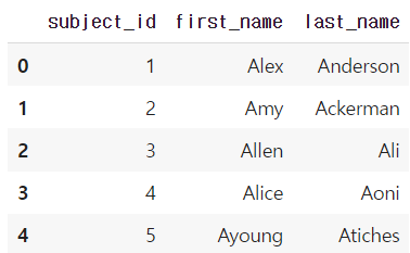
raw_data = {
        'subject_id': ['4', '5', '6', '7', '8'],
        'first_name': ['Billy', 'Brian', 'Bran', 'Bryce', 'Betty'],
        'last_name': ['Bonder', 'Black', 'Balwner', 'Brice', 'Btisan']}
df_b = pd.DataFrame(raw_data, columns = ['subject_id', 'first_name', 'last_name'])
df_b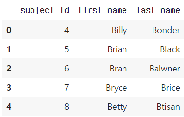
df_new = pd.concat([df_a, df_b])
df_new.reset_index(drop=True)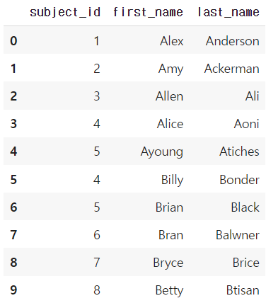
df_a.append(df_b)
df_new = pd.concat([df_a, df_b], axis=1)
df_new.reset_index(drop=True)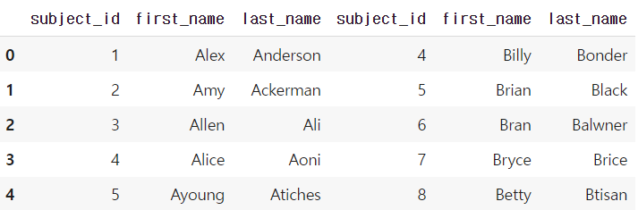
🔹 persistence
▶ Database connection
- Dataloading시 db connection기능을 제공한다.
# Database 연결 코드
import sqlite3 #pymysql <- 설치

conn = sqlite3.connect("./data/flights.db")
cur = conn.cursor()
cur.execute("select * from airlines limit 5;")
results = cur.fetchall()
results
# db 연결 conn을 사용하여 dataframe 생성
df_airplines = pd.read_sql_query("select * from airlines;", conn)
df_airplines
▶ XLS persistence
- Dataframe의 엑셀 추출 코드
- Xls 엔진으로 openpyxls 또는 XlsxWrite 사용
writer = pd.ExcelWriter('./data/df_routes.xlsx', engine='xlsxwriter')
df_routes.to_excel(writer, sheet_name='Sheet1')
▶ Pickle persistence
- 가장 일반적인 python파일 persistence
- to_pickle,read_pickle 함수 사용
df_routes.to_pickle("./data/df_routes.pickle")
df_routes_pickle = pd.read_pickle("./data/df_routes.pickle")
'Python > Numpy | Pandas' 카테고리의 다른 글
| [Pandas] Pandas 공부하기 좋은 자료 (0) | 2023.10.09 |
|---|---|
| [Pandas] str.startswith(), str.endswith(), str.contains() (0) | 2023.06.21 |
| [Numpy] array를 list로 변환 (0) | 2023.01.02 |
| [Numpy] comparisons, boolean&fancy index, numpy data i/o (0) | 2022.12.27 |
| [Numpy] shape, creation, operation 관련 함수 (0) | 2022.12.27 |

