
코딩하는 해맑은 거북이
[Numpy] shape, creation, operation 관련 함수 본문
본 게시물의 내용은 'Numpy(부스트캠프 AI Tech)' 강의를 듣고 작성하였다.
Handling shape
- reshape : Array의 shape의 크기를 element의 갯수는 동일하게 변경함.
* -1 : size를 기반으로 row나 column의 개수 선정해줌
test_matrix = [[1, 2, 3, 4], [1, 2, 5, 8]]
np.array(test_matrix).shape
(2, 4)
np.array(test_matrix).reshape(8,)array([1, 2, 3, 4, 1, 2, 5, 8])
np.array(test_matrix).reshape(4, 2)array([[1, 2],
[3, 4],
[1, 2],
[5, 8]])
np.array(test_matrix).reshape(2, 2, 2)array([[[1, 2],
[3, 4]],
[[1, 2],
[5, 8]]])
np.array(test_matrix).reshape(1, -1)array([[1, 2, 3, 4, 1, 2, 5, 8]])
np.array(test_matrix).reshape(1, -1).shape(1, 8)
np.array(test_matrix).reshape(1, -1, 2)array([[1, 2],
[3, 4],
[1, 2],
[5, 8]])
np.array(test_matrix).reshape(1, -1, 2).shape(1, 4, 2)
- flatten : 다차원 array를 1차원 array로 변환
test_tensor = [[[1,2,3,4], [1,2,5,8]], [[1,2,3,4], [1,2,5,8]]]
np.array(test_tensor).flatten()
array([1, 2, 3, 4, 1, 2, 5, 8, 1, 2, 3, 4, 1, 2, 5, 8])
indexing & slicing
indexing for numpy array
- list와 달리 이차원 배열에서 [0, 0] 표기법을 제공함
- matrix 일 경우 앞은 row, 뒤는 column을 의미함
a = np.array([[1, 2, 3], [4.5, 5, 6]], int)
print(a)
[[1 2 3]
[4 5 6]]
print(a[0,0]) # Two dimensional array representation #1
print(a[0][0]) # Two dimensional array representation #2
1
1
a[0,0] = 12 # Matrix 0,0 에 12 할당
print(a)
[[12 2 3]
[ 4 5 6]]
slicing for numpy array
- list와 달리 행과 열 부분을 나눠서 slicing이 가능함
- matrix의 부분 집합을 추출할 때 유용함
a = np.array([[1, 2, 3, 4, 5], [6, 7, 8, 9, 10]], int)
a[:, 2:]     # 전체 Row의 2열 이상
array([[ 3, 4, 5],
[ 8, 9, 10]])
a[1, 1:3] # 1 Row의 1열 ~ 2열array([7, 8])
a[1:3] # 1 Row ~ 2Row의 전체array([[ 6, 7, 8, 9, 10]])
Creation function
- arange : array의 범위를 지정하여, 값의 list를 생성하는 명령어
np.arange(30)array([ 0, 1, 2, 3, 4, 5, 6, 7, 8, 9, 10, 11, 12, 13, 14, 15, 16, 17, 18, 19, 20, 21, 22, 23, 24, 25, 26, 27, 28, 29])
np.arange(0, 5, 0.5)array([0. , 0.5, 1. , 1.5, 2. , 2.5, 3. , 3.5, 4. , 4.5])
np.arange(30).reshape(5, 6)array([[ 0, 1, 2, 3, 4, 5],
[ 6, 7, 8, 9, 10, 11],
[12, 13, 14, 15, 16, 17],
[18, 19, 20, 21, 22, 23],
[24, 25, 26, 27, 28, 29]])
- zeros : 0으로 가득찬 ndarray 생성
np.zeros(shape=(10,), dtype=np.int8)array([0, 0, 0, 0, 0, 0, 0, 0, 0, 0], dtype=int8)
np.zeros((2, 5))array([[0., 0., 0., 0., 0.],
[0., 0., 0., 0., 0.]])
- ones : 1로 가득찬 ndarray 생성
np.ones(shape=(10,), dtype=np.int8)array([1, 1, 1, 1, 1, 1, 1, 1, 1, 1], dtype=int8)
np.ones((2, 5))array([[1., 1., 1., 1., 1.],
[1., 1., 1., 1., 1.]])
- empty : shape만 주어지고 비어있는 ndarray 생성
( memory initialization 이 되지 않음 - 다른프로그램에서 쓴 값들이 남아있을 수 있음 )
np.empty(shape=(10,), dtype=np.int8)array([1, 1, 1, 1, 1, 1, 1, 1, 1, 1], dtype=int8)
np.empty((3, 5))array([[1.28182605e-316, 3.85371204e-322, 0.00000000e+000, 0.00000000e+000, 0.00000000e+000],
[1.50008929e+248, 4.31174539e-096, 9.80058441e+252, 1.23971686e+224, 1.05249889e-153],
[9.03292329e+271, 9.08366793e+223, 1.06244660e-153, 3.44981369e+175, 6.81019663e-310]])
- somthing_like : 기존 ndarray의 shape 크기 만큼 1, 0 또는 empty array를 반환
test_matrix = np.arange(30).reshape(5, 6)
np.ones_like(test_matrix)
array([[1, 1, 1, 1, 1, 1],
[1, 1, 1, 1, 1, 1],
[1, 1, 1, 1, 1, 1],
[1, 1, 1, 1, 1, 1],
[1, 1, 1, 1, 1, 1]])
- identity : 단위 행렬(i 행렬)을 생성함
np.identity(n=3, dtype=np.int8)array([[1, 0, 0],
[0, 1, 0],
[0, 0, 1]], dtype=int8)
np.identity(5)array([[1., 0., 0., 0., 0.],
[0., 1., 0., 0., 0.],
[0., 0., 1., 0., 0.],
[0., 0., 0., 1., 0.],
[0., 0., 0., 0., 1.]])
- eye : 대각선이 1인 행렬, 시작 index를 k값으로 변경 가능
np.eye(3)array([[1., 0., 0.], [0., 1., 0.], [0., 0., 1.]])
np.eye(3, 5, k=2)array([[0., 0., 1., 0., 0.],
[0., 0., 0., 1., 0.],
[0., 0., 0., 0., 1.]])
np.eye(N=3, M=5, dtype=np.int8)array([[1, 0, 0, 0, 0],
[0, 1, 0, 0, 0],
[0, 0, 1, 0, 0]], dtype=int8)
- diag : 대각 행렬의 값을 추출함
matrix = np.arange(9).reshape(3, 3)
np.diag(matrix)
array([0, 4, 8])
np.diag(matrix, k=1)array([1, 5])
- random sampling : 데이터 분포에 따른 sampling으로 array를 생성
np.random.uniform(0, 1, 10).reshape(2, 5) # 균등분포array([[0.96150938, 0.35115447, 0.70280082, 0.15545921, 0.49814371],
[0.64544034, 0.44062397, 0.4690827 , 0.95977091, 0.31030859]])
np.random.normal(0, 1, 10).reshape(2, 5) # 정규분포array([[-0.93216005, 1.41627827, -0.32963233, -0.35021354, 1.12413161],
[ 1.92946909, 0.6351734 , -0.43239319, -1.70391322, 0.58146431]])
Operation functions
- sum : ndarray의 element들 간의 합을 구함, list의 sum 기능과 동일
test_array = np.arange(1, 11)
test_array.sum(dtype=np.float64)
55.0
- axis : 모든 operation function을 실행할 때 기준이 되는 dimension 축
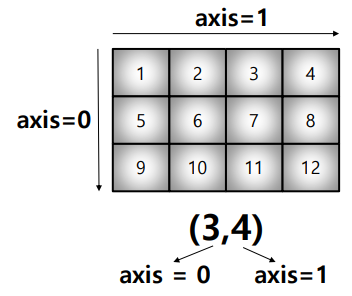
test_array = np.arange(1, 13).reshape(3, 4)
test_array.sum(axis=1), test_array.sum(axis=0)
(array([10, 26, 42]), array([15, 18, 21, 24]))
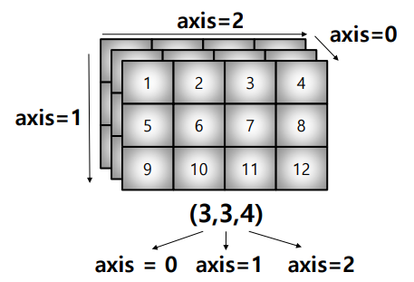
test_tensor = [[[1, 2, 3, 4], [5, 6, 7, 8], [9, 10, 11, 12]],
 [[1, 2, 3, 4], [5, 6, 7, 8], [9, 10, 11, 12]],
 [[1, 2, 3, 4], [5, 6, 7, 8], [9, 10, 11, 12]]]
np.array(test_tensor).shape
(3, 3, 4)
np.array(test_tensor).sum(axis=2)array([[10, 26, 42],
[10, 26, 42],
[10, 26, 42]])
np.array(test_tensor).sum(axis=1)array([[15, 18, 21, 24],
[15, 18, 21, 24],
[15, 18, 21, 24]])
np.array(test_tensor).sum(axis=0)array([[ 3, 6, 9, 12],
[15, 18, 21, 24],
[27, 30, 33, 36]])
- mean & std : ndarray의 element들 간의 평균 또는 표준편차를 반환
test_array = np.arange(1, 13).reshape(3, 4)
test_array.mean(), test_array.mean(axis=0)
(6.5, array([5., 6., 7., 8.]))
test_array.std(), test_array.std(axis=0)(3.452052529534663, array([3.26598632, 3.26598632, 3.26598632, 3.26598632]))
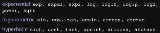
- mathematical functions : 그 외에도 다양한 수학 연산자를 제공함 (np.~ 로 호출)
- concatenate : numpy array를 합치는(붙이는) 함수
* vstack : row 기준으로 붙임
* hstack : column 기준으로 붙임
* concatenate : axis 를 기준으로 붙임 (axis = 0 : row 기준 / axis = 1 : column 기준)
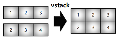
a = np.array([1, 2, 3])
b = np.array([2, 3, 4])
np.vstack((a, b))
array([[1, 2, 3],
[2, 3, 4]])
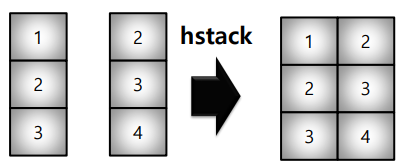
a = np.array([[1], [2], [3]])
b = np.array([[2], [3], [4]])
np.hstack((a, b))
array([[1, 2],
[2, 3],
[3, 4]])
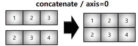
a = np.array([[1, 2, 3]])
b = np.array([[2, 3, 4]])
np.concatenate((a, b), axis=0)
array([[1, 2, 3],
[2, 3, 4]])
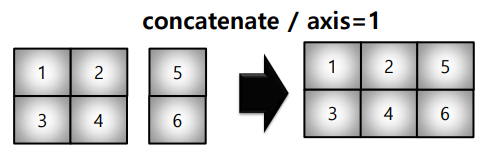
a = np.array([[1, 2], [3, 4]])
b = np.array([[5, 6]])
np.concatenate((a, b.T), axis=1)
array([[1, 2, 5],
[3, 4, 6]])
cf) 차원을 추가하는 방법 2가지
b = np.array([5, 6])  # shape = (2,)
b.reshape(-1, 2)      # shape = (1, 2)
array([[5, 6]])
b = np.array([5, 6])  # shape = (2,)
b[np.newaxis, :]      # shape = (1, 2)
array([[5, 6]])
array operation
- operations b/t arrays : numpy는 array간의 기본적인 사칙 연산을 지원함
test_a = np.array([[1, 2, 3], [4, 5, 6]], float)test_a + test_aarray([[ 2., 4., 6.],
[ 8., 10., 12.]])
test_a - test_aarray([[0., 0., 0.],
[0., 0., 0.]])
test_a * test_aarray([[ 1., 4., 9.],
[16., 25., 36.]])
- 기본 조건 >> Element-wise operations : Array간 shape이 같을 때 일어나는 연산
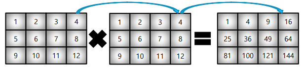
matrix_a = np.arange(1, 13).reshape(3, 4)
matrix_a * matrix_a
array([[ 1, 4, 9, 16],
[ 25, 36, 49, 64],
[ 81, 100, 121, 144]])
- Dot product : Matrix의 기본 연산(내적을 이용한 행렬곱), dot 함수 사용
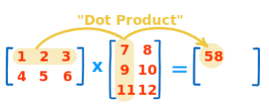
test_a = np.arange(1, 7).reshape(2, 3)
test_b = np.arange(7, 13).reshape(3, 2)
test_a.dot(test_b)
array([[ 58, 64],
[139, 154]])
- transpose : 전치, transpose 또는 T attribute 사용
test_a = np.arange(1, 7).reshape(2, 3)
test_a
array([[1, 2, 3],
[4, 5, 6]])
test_a.transpose()array([[1, 4],
[2, 5],
[3, 6]])
test_a.Tarray([[1, 4],
[2, 5],
[3, 6]])
- broadcasting : shape이 다른 배열 간 연산을 지원하는 기능
test_matrix = np.array([[1, 2, 3], [4, 5, 6]], float)
scalar = 3
test_matrix
array([[1., 2., 3.],
[4., 5., 6.]])
test_matrix + scalararray([[4., 5., 6.],
[7., 8., 9.]])
test_matrix - scalararray([[-2., -1., 0.],
[ 1., 2., 3.]])
test_matrix * scalararray([[ 3., 6., 9.],
[12., 15., 18.]])
test_matrix / 5array([[0.2, 0.4, 0.6],
[0.8, 1. , 1.2]])
test_matrix // 0.2array([[ 4., 9., 14.],
[19., 24., 29.]])
test_matrix ** 2array([[ 1., 4., 9.],
[16., 25., 36.]])
* Scalar-vector 외에도 vector-matrix 간 연산도 가능
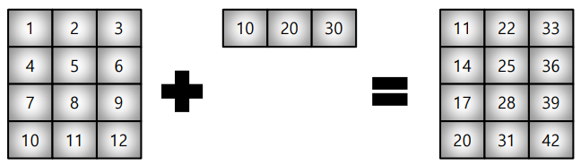
test_matrix = np.arange(1, 13).reshape(4, 3)
test_vector = np.arange(10, 40, 10)
test_matrix + test_vector
array([[11, 22, 33],
[14, 25, 36],
[17, 28, 39],
[20, 31, 42]])
'Python > Numpy | Pandas' 카테고리의 다른 글
| [Numpy] array를 list로 변환 (0) | 2023.01.02 |
|---|---|
| [Numpy] comparisons, boolean&fancy index, numpy data i/o (0) | 2022.12.27 |
| [Numpy] Numpy란, Numpy 특징, ndarray (0) | 2022.12.27 |
| [Numpy] Numpy 배열 생성 방법 (0) | 2021.01.07 |
| [Numpy] Numpy 정의, 설치, 라이브러리 선언 (0) | 2021.01.05 |
